COMPUTER GRAPHICS AND IMAGE PROCESSING LABORATORY

In this blog post, you will find solutions for the COMPUTER GRAPHICS AND IMAGE PROCESSING LABORATORY (21CSL66) course work for the VI semester of VTU university. To follow along, you will need to have up a machine running any flavour of GNULinux OS. We recommend using the GCC compiler for this lab. The solutions have been tested on Ubuntu 22.04 OS. You can find the lab syllabus on the university’s website or here below.

21CSL66 Download

All these solutions have been maintained at the following git repository shown below. If you want to contribute send me a PR.

https://gitlab.com/lab_manuals/current/vi-semester/21csl66_computer_graphics_and_image_processing_laboratory

Installing OpenGL and OpenCV

This lab requires you to use two libraries OpenGL and OpenCV . We will be using C++ for OpenGL and Python for OpenCV. Lets see how to setup the requisite software .

OpenGL Installation

On Ubuntu 22.04, GCC is installed by default all we have to do is install the OpenGL library freeglut. freeglut is a free-software/open-source alternative to the OpenGL Utility Toolkit (GLUT) library. You can install freeglut using the following command.

sudo apt install freeglut3

Now the requisite libraries will be installed, which can be verified as follows.

$ ls -d /usr/include/GL
/usr/include/GL

After getting the necessary development environment setup, Now lets focus on the solutions.

Compilation

To compile use the g++ compiler for C++ code or gcc if you are coding in C language as follows. While compiling one has to link to GL, GLU and glut. Optionally you can redirect the output to the file of your choice as shown below.

$ g++ filename.cpp -lGL -lGLU -lglut -o outputname

OpenCV Installation

As said earlier we would require the Python environment for using OpenCV library. It is recommended to setup the Python environment using the Anconda installer. A detailed procedure can be found here in this following blog.

Setting up Anaconda Python Programming Environment on Ubuntu

After setting up the Anaconda environment we can now install OpenCV using the conda installer.

$ conda install opencv

To verify the installation do the following.

The OpenCV version is contained within a special cv2.__version__ variable, which you can access like this:

$ python
>>> import cv2
>>> cv2.__version__
'4.6.0'

After getting the necessary development environment setup, Now lets focus on the solutions. You can go to the appropriate program by clicking on the links below.

Bresenham’s line drawing technique
Basic geometric operations on the 2D object
Basic geometric operations on the 3D object
2D transformations
3D transformations
Animation effects

Split and Display Image
Rotation, Scaling and Translation on an image
Feature Extraction
Blur and Smoothing
Contour detection
Face Detection

OpenGL

Question 1

Bresenham’s line drawing technique

Develop a program to draw a line using Bresenham’s line drawing technique

C++ Program

#include <GL/glut.h>
#include <iostream>
using namespace std;

// Bresenham's line drawing algorithm
void drawLine(int x0, int y0, int x1, int y1) {
    int dx = abs(x1 - x0);
    int dy = abs(y1 - y0);
    int sx = (x0 < x1) ? 1 : -1;
    int sy = (y0 < y1) ? 1 : -1;
    int err = dx - dy;

    while (true) {
        glBegin(GL_POINTS);
        glVertex2i(x0, y0);
        glEnd();

        if (x0 == x1 && y0 == y1) break;

        int e2 = 2 * err;
        if (e2 > -dy) {
            err -= dy;
            x0 += sx;
        }
        if (e2 < dx) {
            err += dx;
            y0 += sy;
        }
    }
}

// OpenGL display callback
void display() {
    int x1, x2, y1, y2;

    cout << "Enter coordinates for x1 and y1" << endl;
    cin >> x1 >> y1;
    cout << "Enter coordinates for x2 and y2" << endl;
    cin >> x2 >> y2;

    glClear(GL_COLOR_BUFFER_BIT);

    // Draw line using Bresenham's algorithm
    glColor3f(1.0f, 1.0f, 1.0f);
    drawLine(x1, y1, x2, y2);

    glFlush();
}

// OpenGL initialization
void initializeOpenGL(int argc, char** argv) {
    glutInit(&argc, argv);
    glutInitDisplayMode(GLUT_SINGLE | GLUT_RGB);
    glutInitWindowSize(800, 600);
    glutCreateWindow("Bresenham's Line Algorithm");

    glClearColor(0.0f, 0.0f, 0.0f, 1.0f);
    glMatrixMode(GL_PROJECTION);
    glLoadIdentity();
    gluOrtho2D(0, 800, 0, 600);

    glutDisplayFunc(display);
}

// Main function
int main(int argc, char** argv) {

    initializeOpenGL(argc, argv);

    glutMainLoop();

    return 0;
}

In this program:

We include for GLUT functions and OpenGL headers.
The drawLine function implements Bresenham’s line drawing algorithm, just like in the previous example.
The display function is the GLUT display callback, where we clear the screen and draw the line using drawLine.
The initializeOpenGL function sets up the GLUT window and OpenGL context. It specifies the display mode, window size, and title. It also sets up the projection matrix and registers the display callback.
In main, we initialize the OpenGL context using initializeOpenGL and start the GLUT main loop with glutMainLoop().
Compile this program with a C++ compiler that links against GLUT and OpenGL libraries. When you run the compiled program, it should open an OpenGL window displaying a white line drawn using Bresenham’s algorithm from (50, 50) to (500, 500) given as input from the user. Adjust the window size and line coordinates as needed.

Output

$ g++ 01_Bresenham.cpp -lGL -lGLU -lglut -o 01_Bresenham.x

$ ./01_Bresenham.x 
Enter coordinates for x1 and y1
50 50
Enter coordinates for x1 and y1
500 500

Question 2

Basic geometric operations on the 2D object

Develop a program to demonstrate basic geometric operations on the 2D object

C++ Program

#include <GL/glut.h>
#include <iostream>

// Global variables
int width = 800;
int height = 600;
float rectWidth = 100.0f;
float rectHeight = 50.0f;
float rectPositionX = (width - rectWidth) / 2.0f;
float rectPositionY = (height - rectHeight) / 2.0f;
float rotationAngle = 0.0f;
float scaleFactor = 1.0f;

// Function to draw a rectangle
void drawRectangle(float x, float y, float width, float height) {
    glBegin(GL_POLYGON);
    glVertex2f(x, y);
    glVertex2f(x + width, y);
    glVertex2f(x + width, y + height);
    glVertex2f(x, y + height);
    glEnd();
}

// Function to handle display
void display() {
    glClear(GL_COLOR_BUFFER_BIT);

    glMatrixMode(GL_MODELVIEW);
    glLoadIdentity();

    // Apply transformations
    glTranslatef(rectPositionX, rectPositionY, 0.0f);
    glRotatef(rotationAngle, 0.0f, 0.0f, 1.0f);
    glScalef(scaleFactor, scaleFactor, 1.0f);

    // Draw rectangle
    glColor3f(1.0f, 0.0f, 0.0f); // Red color
    drawRectangle(0.0f, 0.0f, rectWidth, rectHeight);

    glFlush();
}

// Function to handle keyboard events
void keyboard(unsigned char key, int x, int y) {
    switch (key) {
        case 't':
            // Translate the rectangle by 10 units in the x-direction
            rectPositionX += 10.0f;
            break;
        case 'r':
            // Rotate the rectangle by 10 degrees clockwise
            rotationAngle += 10.0f;
            break;
        case 's':
            // Scale the rectangle by 10% (scaleFactor = 1.1f)
            scaleFactor *= 1.1f;
            break;
        case 'u':
            // Reset transformations (translate back to center, reset rotation and scaling)
            rectPositionX = (width - rectWidth) / 2.0f;
            rectPositionY = (height - rectHeight) / 2.0f;
            rotationAngle = 0.0f;
            scaleFactor = 1.0f;
            break;
        case 27: // Escape key to exit
            exit(0);
            break;
    }

    glutPostRedisplay(); // Trigger a redraw
}

// Function to initialize OpenGL
void initializeOpenGL(int argc, char** argv) {
    glutInit(&argc, argv);
    glutInitDisplayMode(GLUT_SINGLE | GLUT_RGB);
    glutInitWindowSize(width, height);
    glutCreateWindow("Geometric Operations in 2D");

    glClearColor(1.0f, 1.0f, 1.0f, 1.0f); // White background
    glMatrixMode(GL_PROJECTION);
    glLoadIdentity();
    gluOrtho2D(0, width, 0, height);

    glutDisplayFunc(display);
    glutKeyboardFunc(keyboard);
}

// Main function
int main(int argc, char** argv) {
    initializeOpenGL(argc, argv);
    glutMainLoop();
    return 0;
}

In this program:

The glMatrixMode(GL_PROJECTION) and glLoadIdentity() in the initializeOpenGL function ensure that the projection matrix is properly set up.
We define a simple drawRectangle function that draws a rectangle using OpenGL primitives.
The display function is responsible for rendering the scene. It applies translation (glTranslatef), rotation (glRotatef), and scaling (glScalef) transformations to the rectangle before drawing it.
The glTranslatef, glRotatef, and glScalef calls in the display function are applied correctly within the GL_MODELVIEW matrix mode.
The glColor3f(1.0f, 0.0f, 0.0f) call sets the drawing color to red (RGB values: 1.0, 0.0, 0.0).
Keyboard input is handled by the keyboard function. Pressing keys ‘t’, ‘r’, ‘s’, and ‘u’ triggers translation, rotation, scaling, and reset operations, respectively.
The initializeOpenGL function sets up the GLUT window and initializes OpenGL settings.
In main, we initialize the OpenGL context using initializeOpenGL and start the GLUT main loop.

To compile and run this program, make sure you have GLUT installed and set up in your development environment. Compile the program using a C++ compiler that links against GLUT and OpenGL libraries (e.g., using -lglut -lGL -lGLU flags). When you run the compiled program, a window will appear displaying a red rectangle. Use the keyboard keys (‘t’, ‘r’, ‘s’, ‘u’) to perform translation, rotation, scaling, and reset operations on the rectangle interactively.

$ g++ 02_Geometric_2D.cpp -lGL -lGLU -lglut -o 02_Geometric_2D.x

$ ./02_Geometric_2D.x

Question 3

Basic geometric operations on the 3D object

Develop a program to demonstrate basic geometric operations on the 3D object

To demonstrate basic geometric operations on a 3D object using GLUT (OpenGL Utility Toolkit), we can create a program that allows you to perform translation, rotation, and scaling operations interactively on a simple 3D object (e.g., a cube). Below is an example program written in C++ using GLUT that demonstrates these geometric transformations on a 3D cube.

C++ Program

#include <GL/glut.h>
#include <iostream>

// Global variables
int width = 800;
int height = 600;
GLfloat rotationX = 0.0f;
GLfloat rotationY = 0.0f;
GLfloat scale = 1.0f;

// Function to draw a cube
void drawCube() {
    glBegin(GL_QUADS);

    // Front face
    glColor3f(1.0f, 0.0f, 0.0f); // Red
    glVertex3f(-0.5f, -0.5f, 0.5f);
    glVertex3f(0.5f, -0.5f, 0.5f);
    glVertex3f(0.5f, 0.5f, 0.5f);
    glVertex3f(-0.5f, 0.5f, 0.5f);

    // Back face
    glColor3f(0.0f, 1.0f, 0.0f); // Green
    glVertex3f(-0.5f, -0.5f, -0.5f);
    glVertex3f(-0.5f, 0.5f, -0.5f);
    glVertex3f(0.5f, 0.5f, -0.5f);
    glVertex3f(0.5f, -0.5f, -0.5f);

    // Top face
    glColor3f(0.0f, 0.0f, 1.0f); // Blue
    glVertex3f(-0.5f, 0.5f, -0.5f);
    glVertex3f(-0.5f, 0.5f, 0.5f);
    glVertex3f(0.5f, 0.5f, 0.5f);
    glVertex3f(0.5f, 0.5f, -0.5f);

    // Bottom face
    glColor3f(1.0f, 1.0f, 0.0f); // Yellow
    glVertex3f(-0.5f, -0.5f, -0.5f);
    glVertex3f(0.5f, -0.5f, -0.5f);
    glVertex3f(0.5f, -0.5f, 0.5f);
    glVertex3f(-0.5f, -0.5f, 0.5f);

    // Right face
    glColor3f(1.0f, 0.0f, 1.0f); // Magenta
    glVertex3f(0.5f, -0.5f, -0.5f);
    glVertex3f(0.5f, 0.5f, -0.5f);
    glVertex3f(0.5f, 0.5f, 0.5f);
    glVertex3f(0.5f, -0.5f, 0.5f);

    // Left face
    glColor3f(0.0f, 1.0f, 1.0f); // Cyan
    glVertex3f(-0.5f, -0.5f, -0.5f);
    glVertex3f(-0.5f, -0.5f, 0.5f);
    glVertex3f(-0.5f, 0.5f, 0.5f);
    glVertex3f(-0.5f, 0.5f, -0.5f);

    glEnd();
}

// Function to handle display
void display() {
    glClear(GL_COLOR_BUFFER_BIT | GL_DEPTH_BUFFER_BIT);

    glMatrixMode(GL_MODELVIEW);
    glLoadIdentity();

    // Apply transformations
    glTranslatef(0.0f, 0.0f, -3.0f);
    glRotatef(rotationX, 1.0f, 0.0f, 0.0f);
    glRotatef(rotationY, 0.0f, 1.0f, 0.0f);
    glScalef(scale, scale, scale);

    // Draw cube
    drawCube();

    glutSwapBuffers();
}

// Function to handle keyboard events
void keyboard(unsigned char key, int x, int y) {
    switch (key) {
        case 'x':
            rotationX += 5.0f;
            break;
        case 'X':
            rotationX -= 5.0f;
            break;
        case 'y':
            rotationY += 5.0f;
            break;
        case 'Y':
            rotationY -= 5.0f;
            break;
        case '+':
            scale += 0.1f;
            break;
        case '-':
            if (scale > 0.1f)
                scale -= 0.1f;
            break;
        case 27: // Escape key to exit
            exit(0);
            break;
    }

    glutPostRedisplay(); // Trigger a redraw
}

// Function to initialize OpenGL
void initializeOpenGL(int argc, char** argv) {
    glutInit(&argc, argv);
    glutInitDisplayMode(GLUT_DOUBLE | GLUT_RGB | GLUT_DEPTH);
    glutInitWindowSize(width, height);
    glutCreateWindow("Geometric Operations in 3D");

    glEnable(GL_DEPTH_TEST);
    glClearColor(1.0f, 1.0f, 1.0f, 1.0f); // White background

    glMatrixMode(GL_PROJECTION);
    glLoadIdentity();
    gluPerspective(45.0f, (float)width / (float)height, 1.0f, 100.0f);

    glutDisplayFunc(display);
    glutKeyboardFunc(keyboard);
}

// Main function
int main(int argc, char** argv) {
    initializeOpenGL(argc, argv);
    glutMainLoop();
    return 0;
}

In this program:

We define a drawCube function that draws a simple cube using GL_QUADS for each face.
The display function sets up the model-view matrix and applies translation (glTranslatef), rotation (glRotatef), and scaling (glScalef) transformations to the cube before drawing it.
Keyboard input is handled by the keyboard function. Pressing keys ‘x’, ‘X’, ‘y’, and ‘Y’ rotates the cube around the X and Y axes, while ‘+’ and ‘-‘ keys scale the cube up and down, respectively.
The initializeOpenGL function sets up the GLUT window, initializes OpenGL settings (including depth testing for 3D rendering), and registers display and keyboard callback functions.
The main function initializes the OpenGL context using initializeOpenGL and starts the GLUT main loop.

Compile and run this program, and you should see a window displaying a rotating and scalable cube. Use the keyboard keys (‘x’, ‘X’, ‘y’, ‘Y’, ‘+’, ‘-‘) to perform rotation and scaling operations on the cube interactively. The modifications made in this version should ensure that the cube is visible and that the geometric transformations work as expected in a 3D context.

Output

$ g++ 03_Geometric_3D.cpp -lglut -lGLU -lGL -o 03_Geometric_3D.x

$ ./03_Geometric_3D.x

Question 4

2D transformations

Develop a program to demonstrate 2D transformation on basic objects

C++ Program

Output

Question 5

3D transformations

Develop a program to demonstrate 3D transformation on 3D objects

C++ Program

Output

Question 6

Animation effects

Develop a program to demonstrate Animation effects on simple objects.

C++ Program

#include <GL/glut.h>
#include <math.h>
#include <stdlib.h>

const double TWO_PI = 6.2831853;
GLsizei winWidth = 500, winHeight = 500;
GLuint regHex;
static GLfloat rotTheta = 0.0;

// Initial display window size.
// Define name for display list.
class scrPt {
	public:
	GLint x, y;
};

static void init(void)
{
	scrPt hexVertex;
	GLdouble hexTheta;
	GLint k;
	glClearColor(1.0, 1.0, 1.0, 0.0);
	/* Set up a display list for a red regular hexagon.
	* Vertices for the hexagon are six equally spaced
	* points around the circumference of a circle.
	*/
	regHex = glGenLists(1);
	glNewList(regHex, GL_COMPILE);
	glColor3f(1.0, 0.0, 0.0);
	glBegin(GL_POLYGON);
	for(k = 0; k < 6; k++) {
		hexTheta = TWO_PI * k / 6;
		hexVertex.x = 150 + 100 * cos(hexTheta);
		hexVertex.y = 150 + 100 * sin(hexTheta);
		glVertex2i(hexVertex.x, hexVertex.y);
	}
	glEnd( );
	glEndList( );
}

void displayHex(void)
{
	glClear(GL_COLOR_BUFFER_BIT);
	glPushMatrix( );
	glRotatef(rotTheta, 0.0, 0.0, 1.0);
	glCallList(regHex);
	glPopMatrix( );
	glutSwapBuffers( );
	glFlush( );
}

void rotateHex(void)
{
	rotTheta += 3.0;
	if(rotTheta > 360.0)
	rotTheta -= 360.0;
	glutPostRedisplay( );
}
void winReshapeFcn(GLint newWidth, GLint newHeight)
{
	glViewport(0, 0,(GLsizei) newWidth,(GLsizei) newHeight);
	glMatrixMode(GL_PROJECTION);
	glLoadIdentity( );
	gluOrtho2D(-320.0, 320.0, -320.0, 320.0);
	glMatrixMode(GL_MODELVIEW);
	glLoadIdentity( );
	glClear(GL_COLOR_BUFFER_BIT);
}
void mouseFcn(GLint button, GLint action, GLint x, GLint y)
{
	switch(button) {
		case GLUT_MIDDLE_BUTTON:
			// Start the rotation.
			if(action == GLUT_DOWN)
				glutIdleFunc(rotateHex);
			break;
		case GLUT_RIGHT_BUTTON:
			// Stop the rotation.
			if(action == GLUT_DOWN)
				glutIdleFunc(NULL);
			break;
		default:
			break;
	}
}

int main(int argc, char** argv)
{
	glutInit(&argc, argv);
	glutInitDisplayMode(GLUT_DOUBLE | GLUT_RGB);
	glutInitWindowPosition(150, 150);
	glutInitWindowSize(winWidth, winHeight);
	glutCreateWindow("Animation Example");
	init( );
	glutDisplayFunc(displayHex);
	glutReshapeFunc(winReshapeFcn);
	glutMouseFunc(mouseFcn);
	glutMainLoop( );
	return 0;
}

The computer-animation features such as Double-buffering operations, if available, are activated using the following GLUT command:
glutInitDisplayMode (GLUT_DOUBLE);
This provides two buffers, called the front buffer and the back buffer, that we can use alternately to refresh the screen display. While one buffer is acting as the refresh buffer for the current display window, the next frame of an animation can be constructed in the other buffer. We specify when the roles of the two buffers are to be interchanged using
glutSwapBuffers ( );

For a continuous animation, we can use
glutIdleFunc (animationFcn);
where parameter animationFcn can be assigned the name of a procedure that is to perform the operations for incrementing the animation parameters. This procedure is continuously executed whenever there are no display-window events that must be processed. The following program illustrates animation, which continuously rotates a regular hexagon in the xy plane about the z axis.

Output

$ g++ 06_Animation.cpp -lGL -lGLU -lglut -o 06_Animation.x

$ ./06_Animation.x

OpenCV

Question 7

Split and Display Image

Write a Program to read a digital image. Split and display image into 4 quadrants, up, down, right and left.

Python Program

import cv2

# Function to split the image into four quadrants
def split_image(image):
    height, width, _ = image.shape
    half_height = height // 2
    half_width = width // 2

    # Split the image into four quadrants
    top_left = image[:half_height, :half_width]
    top_right = image[:half_height, half_width:]
    bottom_left = image[half_height:, :half_width]
    bottom_right = image[half_height:, half_width:]

    return top_left, top_right, bottom_left, bottom_right

# Function to display images
def display_images(images, window_names):
    for img, name in zip(images, window_names):
        cv2.imshow(name, img)

    print("Press any key to terminate.")
    cv2.waitKey(0)
    cv2.destroyAllWindows()

# Read the image
image_path = "image.jpg"  # Replace "image.jpg" with the path to your image
image = cv2.imread(image_path)

if image is None:
    print("Failed to load the image.")
else:
    # Split the image into quadrants
    top_left, top_right, bottom_left, bottom_right = split_image(image)

    # Display the quadrants
    display_images([top_left, top_right, bottom_left, bottom_right], ["Top Left", "Top Right", "Bottom Left", "Bottom Right"])

Defining Functions:

split_image: This function takes an image as input and splits it into four quadrants: top left, top right, bottom left, and bottom right. It calculates the dimensions of the image and then slices the image array accordingly to extract each quadrant.
display_images: This function takes a list of images and a list of window names as input. It displays each image in a separate window with the corresponding window name.

Reading the Image:

We specify the path to the image file that we want to read. If the image is loaded successfully, it is stored in the variable image. If the image loading fails (e.g., due to an incorrect file path), an error message is printed.

Displaying the Quadrants:

The program then calls the display_images function to display each quadrant in a separate window. It passes a list containing the four quadrants as the first argument and a list of window names as the second argument. Each window will display one quadrant of the original image.

cv2.waitKey(0):
- This function waits for a keyboard event indefinitely (0 milliseconds).
- It allows the program to wait until a key is pressed by the user.
- In this program, it’s used to keep the windows open until a key is pressed, preventing them from closing immediately after being displayed.
cv2.destroyAllWindows():
- This function closes all the OpenCV windows.
- It’s used to clean up and close all the windows opened by OpenCV at the end of the program.
- In this program, it’s called after cv2.waitKey(0) to ensure that all windows are closed when the user presses a key to exit the program.

Together, cv2.waitKey(0) and cv2.destroyAllWindows() ensure that the program waits for user input to exit and then closes all windows properly when the program terminates.

Input Image

Click Button to download the input image Download

Output

$ python 07Image_Split.py

Question 8

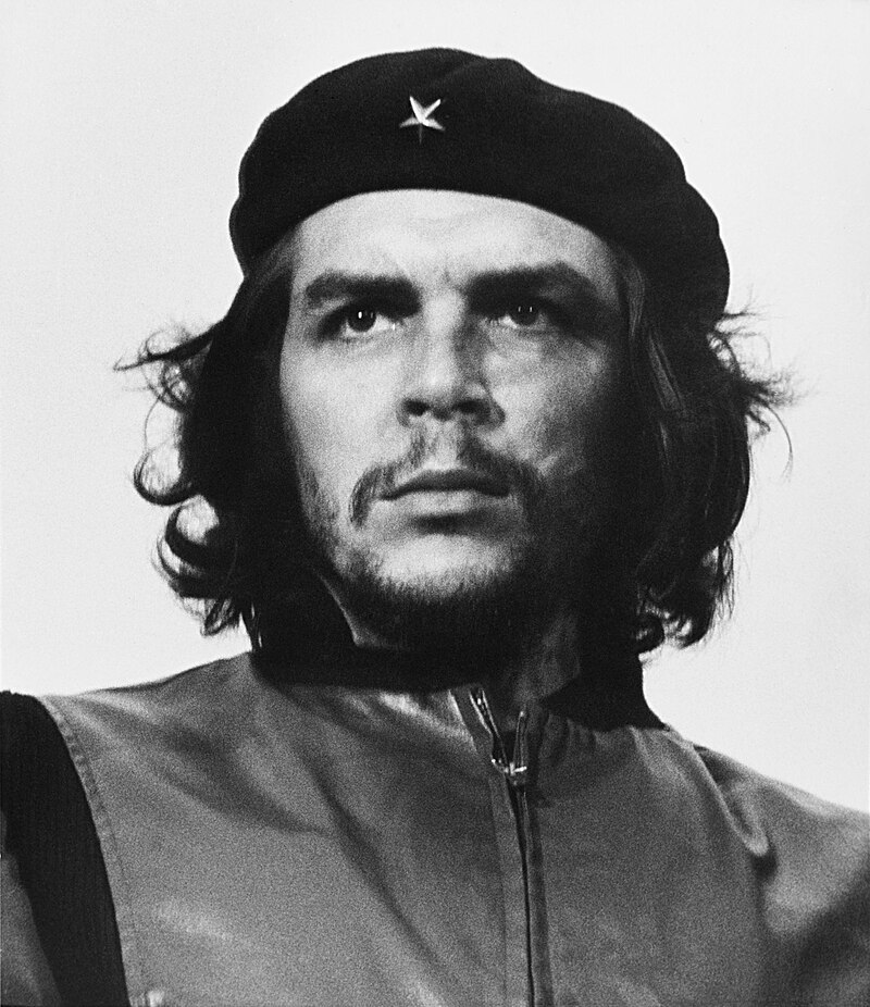
Rotation, Scaling and Translation on an image

Write a program to show rotation, scaling, and translation on an image.

Python Program

import cv2
import numpy as np

# Read the image
image_path = "Che.jpg"  # Replace "your_image.jpg" with the path to your image
image = cv2.imread(image_path)

if image is None:
    print("Failed to load the image.")
else:
    # Display the original image
    cv2.imshow("Original Image", image)

    # Rotation
    angle = 45  # Rotation angle in degrees
    center = (image.shape[1] // 2, image.shape[0] // 2)  # Center of rotation
    rotation_matrix = cv2.getRotationMatrix2D(center, angle, 1.0)  # Rotation matrix
    rotated_image = cv2.warpAffine(image, rotation_matrix, (image.shape[1], image.shape[0]))

    # Scaling
    scale_factor = 0.5  # Scaling factor (0.5 means half the size)
    scaled_image = cv2.resize(image, None, fx=scale_factor, fy=scale_factor)

    # Translation
    translation_matrix = np.float32([[1, 0, 100], [0, 1, -50]])  # Translation matrix (100 pixels right, 50 pixels up)
    translated_image = cv2.warpAffine(image, translation_matrix, (image.shape[1], image.shape[0]))

    # Display the transformed images
    cv2.imshow("Rotated Image", rotated_image)
    cv2.imshow("Scaled Image", scaled_image)
    cv2.imshow("Translated Image", translated_image)

    cv2.waitKey(0)
    cv2.destroyAllWindows()

In this program:

We read an image from a file specified by image_path.
If the image is loaded successfully, we display the original image using cv2.imshow.
We then perform three transformations on the image:
1. Rotation: We rotate the image by an angle of 45 degrees around its center using cv2.getRotationMatrix2D and cv2.warpAffine.
2. Scaling: We scale down the image by a factor of 0.5 using cv2.resize.
3. Translation: We translate the image by 100 pixels to the right and 50 pixels up using a translation matrix and cv2.warpAffine.
Finally, we display the transformed images (rotated_image, scaled_image, and translated_image) using cv2.imshow.
We wait for any key press to close the windows and then use cv2.destroyAllWindows() to clean up and close all OpenCV windows.

You can replace "Che.jpg" with the path to your own image file. Run this script, and you’ll see the original image and the transformed images (rotated, scaled, and translated) displayed in separate windows.

Input Image

Click Button to download the input image Download

Output

$ python 08_TrasnsformImage.py

Question 9

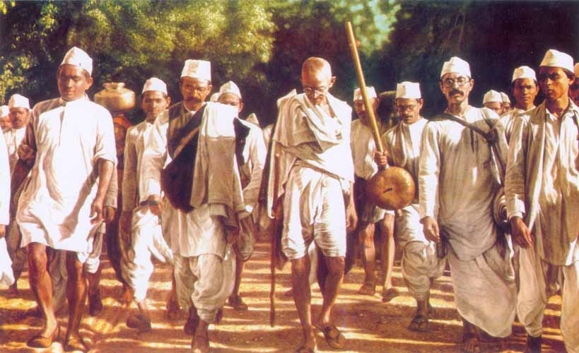
Feature Extraction

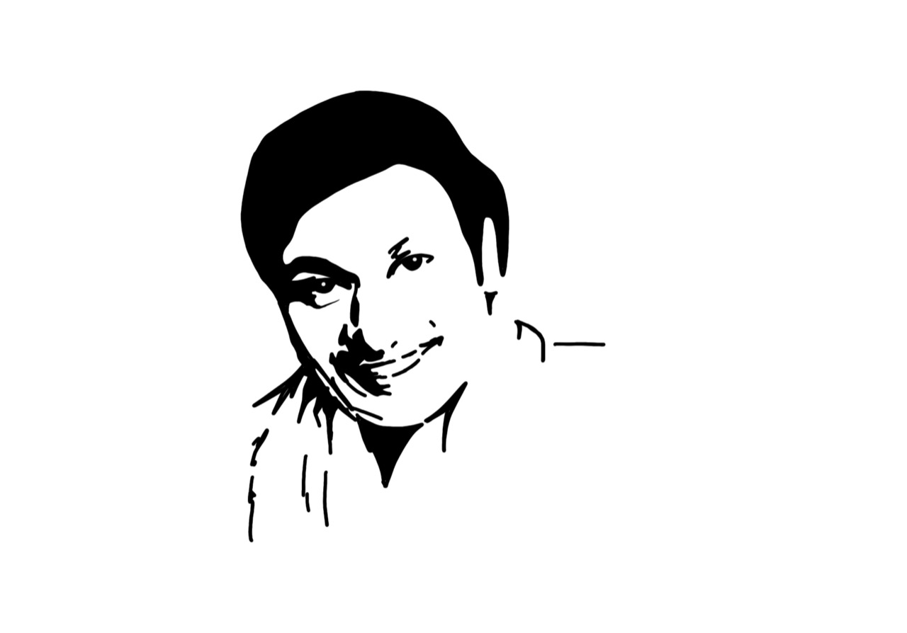
Read an image and extract and display low-level features such as edges, textures using filtering techniques.

Python Program

import cv2
import numpy as np

# Read the image
image_path = "gandhi.jpg"  # Replace "your_image.jpg" with the path to your image
image = cv2.imread(image_path, cv2.IMREAD_GRAYSCALE)

if image is None:
    print("Failed to load the image.")
else:
    # Display the original image
    cv2.imshow("Original Image", image)

    # Apply Sobel filter to extract edges
    sobel_x = cv2.Sobel(image, cv2.CV_64F, 1, 0, ksize=3)
    sobel_y = cv2.Sobel(image, cv2.CV_64F, 0, 1, ksize=3)
    sobel_edges = cv2.magnitude(sobel_x, sobel_y)
    sobel_edges = cv2.normalize(sobel_edges, None, 0, 255, cv2.NORM_MINMAX, dtype=cv2.CV_8U)

    # Display edges extracted using Sobel filter
    cv2.imshow("Edges (Sobel Filter)", sobel_edges)

    # Apply Laplacian filter to extract edges
    laplacian_edges = cv2.Laplacian(image, cv2.CV_64F)
    laplacian_edges = cv2.normalize(laplacian_edges, None, 0, 255, cv2.NORM_MINMAX, dtype=cv2.CV_8U)

    # Display edges extracted using Laplacian filter
    cv2.imshow("Edges (Laplacian Filter)", laplacian_edges)

    # Apply Gaussian blur to extract textures
    gaussian_blur = cv2.GaussianBlur(image, (5, 5), 0)

    # Display image with Gaussian blur
    cv2.imshow("Gaussian Blur", gaussian_blur)

    cv2.waitKey(0)
    cv2.destroyAllWindows()

In this program:

We read an image from a file specified by image_path using cv2.imread.
We convert the image to grayscale since most filtering techniques operate on single-channel images.
We display the original grayscale image using cv2.imshow.
We apply the Sobel filter in both horizontal and vertical directions to extract edges using cv2.Sobel.
We compute the magnitude of gradients obtained from the Sobel filter using cv2.magnitude.
We normalize the result to the range [0, 255] using cv2.normalize.
We display the edges extracted using the Sobel filter.
We apply the Laplacian filter to extract edges using cv2.Laplacian.
We normalize the result to the range [0, 255].
We display the edges extracted using the Laplacian filter.
We apply Gaussian blur to the image to extract textures using cv2.GaussianBlur.
We display the image with Gaussian blur.
We use cv2.waitKey(0) to wait for any key press to close the windows, and cv2.destroyAllWindows() to clean up and close all OpenCV windows.

You can replace "gandhi.jpg" with the path to your own image file. Run this script, and you’ll see the original grayscale image along with the edges extracted using Sobel and Laplacian filters, as well as the image with Gaussian blur applied to it.

Input Image

Click Button to download the input image Download

Output

$ python 09_ImageFeatures.py

Question 10

Blur and Smoothing

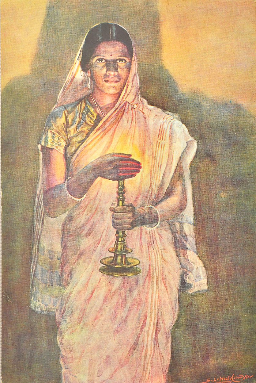
Write a program to blur and smoothing an image.

Blurring and smoothing are common image processing techniques used to reduce noise and detail in images. OpenCV provides various functions to perform blurring and smoothing operations. Below is a Python program using OpenCV to read an image, apply blur and smoothing filters, and display the results:

Python Program

import cv2

# Read the image
image_path = "art.png"  # Replace "your_image.jpg" with the path to your image
image = cv2.imread(image_path)

if image is None:
    print("Failed to load the image.")
else:
    # Display the original image
    cv2.imshow("Original Image", image)

    # Apply blur to the image
    blur_kernel_size = (5, 5)  # Kernel size for blur filter
    blurred_image = cv2.blur(image, blur_kernel_size)

    # Display the blurred image
    cv2.imshow("Blurred Image", blurred_image)

    # Apply Gaussian blur to the image
    gaussian_blur_kernel_size = (5, 5)  # Kernel size for Gaussian blur filter
    gaussian_blurred_image = cv2.GaussianBlur(image, gaussian_blur_kernel_size, 0)

    # Display the Gaussian blurred image
    cv2.imshow("Gaussian Blurred Image", gaussian_blurred_image)

    # Apply median blur to the image
    median_blur_kernel_size = 5  # Kernel size for median blur filter (should be odd)
    median_blurred_image = cv2.medianBlur(image, median_blur_kernel_size)

    # Display the median blurred image
    cv2.imshow("Median Blurred Image", median_blurred_image)

    cv2.waitKey(0)
    cv2.destroyAllWindows()

In this program:

We read an image from a file specified by image_path using cv2.imread.
We display the original image using cv2.imshow.
We apply three different blurring techniques:
1. Blur: We apply a simple averaging filter to the image using cv2.blur.
2. Gaussian Blur: We apply Gaussian blur to the image using cv2.GaussianBlur. This is more effective in reducing noise while preserving edges compared to simple blur.
3. Median Blur: We apply median blur to the image using cv2.medianBlur. This is effective in removing salt-and-pepper noise.
We display the blurred images using cv2.imshow.
We use cv2.waitKey(0) to wait for any key press to close the windows, and cv2.destroyAllWindows() to clean up and close all OpenCV windows.

You can replace "art.png" with the path to your own image file. Run this script, and you’ll see the original image along with the images after applying different blur and smoothing filters.

Input Image

Click Button to download the input image Download

Output

$ python3 10_Blur_Smooth_image.py

Question 11

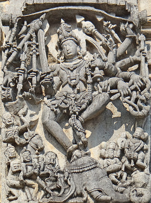
Contour detection

Write a program to contour an image.

Contour detection is a fundamental image processing technique used to find and outline the shapes of objects within an image. OpenCV provides functions to detect contours in images efficiently. Below is a Python program using OpenCV to read an image, detect contours, and draw them on the original image:

Python Program

import cv2

# Read the image
image_path = "annavru.jpeg"  # Replace "your_image.jpg" with the path to your image
image = cv2.imread(image_path)

if image is None:
    print("Failed to load the image.")
else:
    # Convert the image to grayscale
    gray_image = cv2.cvtColor(image, cv2.COLOR_BGR2GRAY)

    # Apply adaptive thresholding
    _, thresh = cv2.threshold(gray_image, 0, 255, cv2.THRESH_BINARY_INV + cv2.THRESH_OTSU)

    # Find contours in the thresholded image
    contours, _ = cv2.findContours(thresh, cv2.RETR_EXTERNAL, cv2.CHAIN_APPROX_SIMPLE)

    # Draw contours on the original image
    contour_image = image.copy()
    cv2.drawContours(contour_image, contours, -1, (0, 255, 0), 2)  # Draw all contours with green color and thickness 2

    # Display the original image with contours
    cv2.imshow("Image with Contours", contour_image)

    cv2.waitKey(0)
    cv2.destroyAllWindows()

In this program:

We read an image from a file specified by image_path using cv2.imread.
We convert the image to grayscale using cv2.cvtColor.
We apply adaptive thresholding (cv2.threshold) to create a binary image where the regions of interest are highlighted.
We find contours in the thresholded image.
We find contours in the thresholded image using cv2.findContours. The cv2.RETR_EXTERNAL flag retrieves only the external contours, and cv2.CHAIN_APPROX_SIMPLE compresses horizontal, vertical, and diagonal segments and leaves only their end points.
We draw the detected contours on a copy of the original image using cv2.drawContours. The contours are drawn with green color and thickness 2.
We display the original image with contours using cv2.imshow.
We use cv2.waitKey(0) to wait for any key press to close the window, and cv2.destroyAllWindows() to clean up and close all OpenCV windows.

You can replace "annavru.jpeg" with the path to your own image file. Run this script, and you’ll see the original image with the detected

Input Image

Click Button to download the input image Download

Output

$ python 11_Contour_Detect.py

Question 12

Face Detection

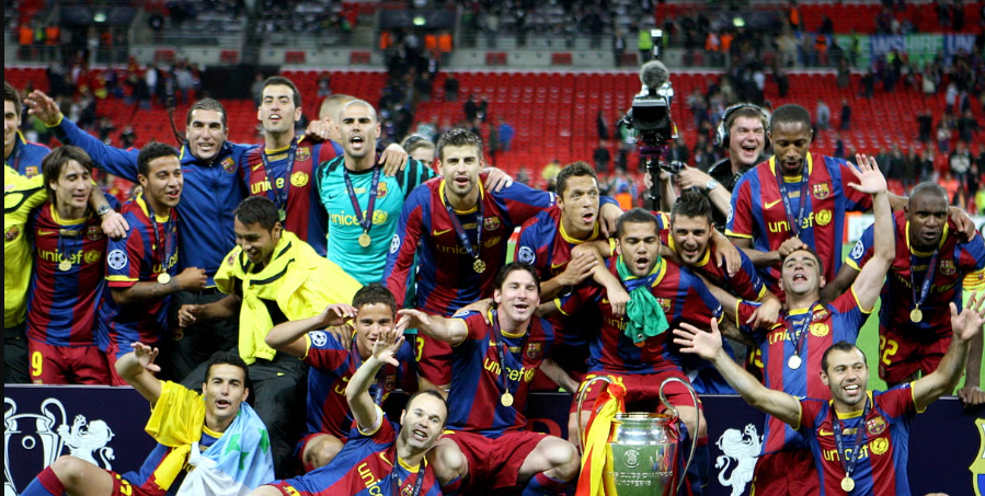
Write a program to detect a face/s in an image.

Python Program

import cv2

# Load the pre-trained Haar Cascade classifier for face detection
face_cascade = cv2.CascadeClassifier('./haarcascades/haarcascade_frontalface_default.xml')

# Read the image
image_path = "ucl.png"  # Replace "ucl.png" with the path to your image
image = cv2.imread(image_path)

if image is None:
    print("Failed to load the image.")
else:
    # Convert the image to grayscale
    gray_image = cv2.cvtColor(image, cv2.COLOR_BGR2GRAY)

    # Detect faces in the image
    faces = face_cascade.detectMultiScale(gray_image, scaleFactor=1.1, minNeighbors=5, minSize=(30, 30))

    # Draw rectangles around the detected faces
    for (x, y, w, h) in faces:
        cv2.rectangle(image, (x, y), (x+w, y+h), (0, 255, 0), 2)

    # Display the image with detected faces
    cv2.imshow("Image with Detected Faces", image)
    cv2.waitKey(0)
    cv2.destroyAllWindows()

Input Image

Click Button to download the input image Download

Output

$ python 12_Face_Detect.py

If you are also looking for other Lab Manuals, head over to my following blog :

VTU Lab Manuals using FOSS

Prabodh C P

Prabodh C P is a faculty in the Dept of CSE SIT, Tumkur and also currently a Research Scholar pursuing PhD in IIT Hyderabad. He conducts online classes for C, C++, Python. For more info call +919392302100

3 Comments

Pawan S says:

May 31, 2024 at 9:22 AM

What about program 4 and program 5 in CGlab is that similar to previous programs

1. Prabodh C P says:
  
  May 31, 2024 at 9:32 AM
  
  I don’t see the difference between them and the two previous programs. The questions are not clear. Hence I have left them empty
  
2. Prabodh C P says:
  
  May 31, 2024 at 9:34 AM
  
  If someone could clarify the same, then I can provide the solution. The question is not specified properly.

Installing OpenGL and OpenCV

OpenGL Installation

OpenCV Installation

OpenGL

Question 1

Bresenham’s line drawing technique

C++ Program

Output

Question 2

Basic geometric operations on the 2D object

C++ Program

Question 3

Basic geometric operations on the 3D object

C++ Program

Output

Question 4

2D transformations

C++ Program

Output

Question 5

3D transformations

C++ Program

Output

Question 6

Animation effects

C++ Program

Output

OpenCV

Question 7

Split and Display Image

Python Program

Input Image

Output

Question 8

Rotation, Scaling and Translation on an image

Python Program

Input Image

Output

Question 9

Feature Extraction

Python Program

Input Image

Output

Question 10

Blur and Smoothing

Python Program

Input Image

Output

Question 11

Contour detection

Python Program

Input Image

Output

Question 12

Face Detection

Python Program

Input Image

Output

Related

Prabodh C P

Related Posts

Full Stack Web Development – 21CS62

MongoDB Lab Manual – BDS456B

Artificial Intelligence Lab Component (BAD402)

3 Comments

Leave a Reply Cancel reply